Transformations

Start again by building the following simple planar structure

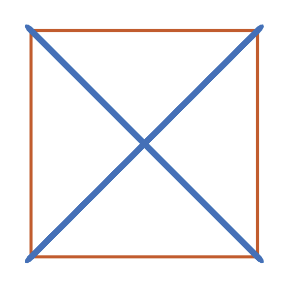
with the following code:

import numpy as np
from tnsgrt.structure import Structure

nodes = np.array([[0,0,0], [0,1,0], [2,1,0], [2,0,0]]).transpose()
members = np.array([[0,1], [1,2], [2,3], [3,0], [0,2], [1,3]]).transpose()
s0 = Structure(nodes, members, number_of_strings=4)

from matplotlib import pyplot as plt
from tnsgrt.plotter.matplotlib import MatplotlibPlotter
%matplotlib widget

plotter = MatplotlibPlotter()
plotter.plot(s0)
fig, ax = plotter.get_handles()
ax.view_init(90,-90)
ax.axis('equal')
ax.axis('off')
plt.show()

Let’s also calculate forces to keep the structure in equilibrium

s0.equilibrium()

which results in force coefficients

s0.member_properties['lambda_']

with the same magnitude in all members:

  1.0
  1.0
  1.0
  1.0
 -1.0
 -1.0
Name: lambda_, dtype: float64

Geometric transformations

Structures support many common geometric transformation. For example,

from tnsgrt import structure
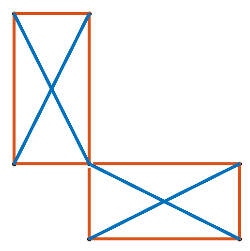
s1 = structure.rotate(s0, np.pi/2*np.array([0,0,1])).translate(np.array([0,1,0]))

performs the following operations:

copy the structure and rotate 90 degrees around the z-axis, and
translate one unit in the direction of the y-axis

Note that geometric operations can be chained.

The transformed structure is plotted jointly with the original structure in the following figure:

produced by the code:

plotter = MatplotlibPlotter()
plotter.plot(s0, s1)
_, ax = plotter.get_handles()
ax.view_init(90,-90)
ax.axis('equal')
ax.axis('off')
plt.show()

Merging Structures

It is also possible to merge various structure while consolidating nodes and members.

Start again by copying and translating the basic planar structure:

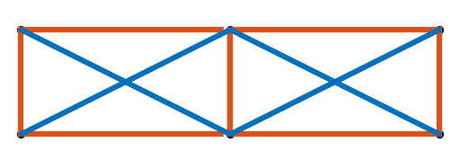
s2 = structure.translate(s0, np.array([2,0,0]))

The result is a structure that has two coincident nodes and one overlapping string. This is visualized in the next figure.

generated by the code:

plotter = MatplotlibPlotter()
plotter.plot(s0, s2)
_, ax = plotter.get_handles()
ax.view_init(90,-90)
ax.axis('equal')
ax.axis('off')
plt.show()

The module function tnsgrt.structure.merge() merges the given structures into a new one

s3 = structure.merge(s2, s0)

The resulting structure, stored in s3, is a structure that is the union of the two given structures, with 8 nodes, 4 bars, and 8 strings. Two pairs of nodes in the structure, namely the pairs (0, 7) and (1, 6),

s3.nodes[:,[0, 7, 1, 6]]

are located in the exact same spatial position:

array([[2., 2., 2., 2.],
       [0., 0., 1., 1.],
       [0., 0., 0., 0.]])

After calling tnsgrt.structure.Structure.merge_close_nodes()

s3.merge_close_nodes()

those two pairs of “close nodes” are merged into single nodes, resulting in a structure with only 6 nodes:

s3.nodes

which are:

array([[2., 2., 4., 4., 0., 0.],
       [0., 1., 1., 0., 0., 1.],
       [0., 0., 0., 0., 0., 0.]])

After merging the close nodes, the structure still has 8 members, with one pair of such members, the members (0, 8), now connected to the exact same pair of nodes:

s3.members[:, [0, 8]]

connecting nodes 0 to 1::

array([[0, 1],
      [1, 0]])

Those members are still independent, each one carrying a suitable set of physical parameters, for example their equilibrium force coefficient, force, and mass:

s3.get_member_properties([0, 8], 'lambda_', 'force', 'mass')

which reveals:

   lambda_  force  mass
0      1.0    1.0   1.0
8      1.0    1.0   1.0

Next we will merge those overlapping members. But before we do that, let’s first add one tag to one of the overlapping members to illustrate what happens during the member merging process.

s3.add_member_tag('redundant', 8)

The overlapping members are now joined by the method tsnsgr.structure.Structure.merge_overlapping_members()

s3.merge_overlapping_members(verbose=True)

This operation removes the overlapping string, resulting in a structure with 6 nodes, 4 bars and 7 strings:

s3.members

located at:

array([[0, 1, 2, 3, 0, 1, 4, 5, 0, 4, 5],
       [1, 2, 3, 0, 2, 3, 5, 1, 4, 1, 0]])

In the new compact structure, member 0 is the one connecting nodes (0, 1) as shown by

s3.members

which produces:

array([[0, 1, 2, 3, 0, 1, 4, 5, 0, 4, 5],
       [1, 2, 3, 0, 2, 3, 5, 1, 4, 1, 0]])

When the members were merged, their tags were also merged, so that the tag redudant now belongs to member 0:

s3.get_members_by_tag('redundant')

now returns:

array([0])

Their physical parameters where also combined:

s3.get_member_properties(0, 'lambda_', 'force', 'mass')

to produce:

lambda_    2.0
force      2.0
mass       2.0
Name: 0, dtype: object

where the other strings in the structure

s3.get_member_properties(s2.get_members_by_tag('string'), 'lambda_', 'force', 'mass')

remain the same:

   lambda_  force  mass
    2.0    2.0   2.0
    1.0    2.0   1.0
    1.0    1.0   1.0
    1.0    2.0   1.0

Of course the geometry of the structure remains the same as shown in the figure

produced by the code:

plotter = MatplotlibPlotter()
plotter.plot(s3)
_, ax = plotter.get_handles()
ax.view_init(90,-90)
ax.axis('equal')
ax.axis('off')
plt.show()