The structure of Structures

The prisms seen in the quick start are members of tnsgrt.structure.Structure. In fact, tnsgrt.prism.Prism overloads only the constructor of tnsgrt.structure.Structure, which provides most of the functionality.

Construction

Object of class tnsgrt.structure.Structure are composed of nodes and members. Nodes are 3 x n numpy arrays:

import numpy as np
nodes = np.array([[0,0,0],[0,1,0],[1,0,0],[1,1,0]]).transpose()

Members are bars or strings, which are specified by a 2 x m array with the indices of the nodes that define the members, as in:

members = np.array([[0,1],[1,2],[2,3],[3,0],[0,2],[1,3]]).transpose()

Nodes and members are then combined to build a tnsgrt.structure.Structure:

from tnsgrt import Structure
s = Structure(nodes, members, number_of_strings=4)

The parameter number_of_strings = 4 means that the first four members are to be considered strings.

As before, the resulting structure can be plotted using tnsgrt.plotter.MatplotlibPlotter:

from tnsgrt.plotter.matplotlib import MatplotlibPlotter
plotter = MatplotlibPlotter()
plotter.plot(s)
fig, ax = plotter.get_handles()
ax.view_init(90,-90)
ax.axis('equal')
ax.axis('off')
plt.show()

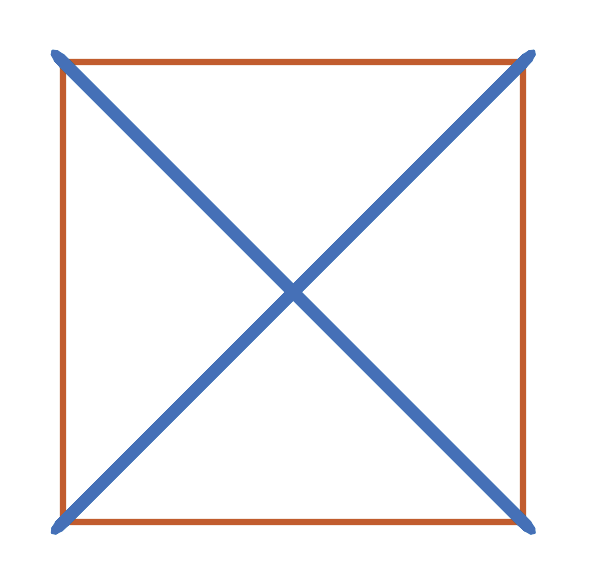
to visualize the resulting planar tensegrity structure below:

Quite often, it is useful to view and modify the data stored in a Structure. The following examples show several ways of doing that.

Nodes and members

A string representation of a Structure displays its number of nodes, number of bars, and number of strings. Typing

print(s)

produces:

Structure with 4 nodes, 2 bars and 4 strings

A Structure has as attributes nodes,

s.nodes

which is a 3 x n numpy array

array([[0., 0., 1., 1.],
       [0., 1., 1., 0.],
       [0., 0., 0., 0.]])

storing the Structure’s nodes in its columns, and members

s.members

which is a 2 x m numpy array:

array([[0, 1, 2, 3, 0, 1],
       [1, 2, 3, 0, 2, 3]], dtype=int64)

storing the Structure’s members. Each column of member stores the indices of the nodes to which the ends of a bar or of a string is connected to.

The values of nodes can be accessed or modified using the convenience methods tnsgrt.structure.Structure.get_node_values() and tnsgrt.structure.Structure.set_node_values(). For example:

s.set_node_values([2, 3], np.array([[2, 1, 0], [2, 0, 0]]).transpose())

modify the location of nodes 2 and 3, and

s.get_node_values([2, 3])

retrieves the updated values:

array([[2., 2.],
       [1., 0.],
       [0., 0.]])

The change is reflected in the structure geometry, which now looks as in the new figure

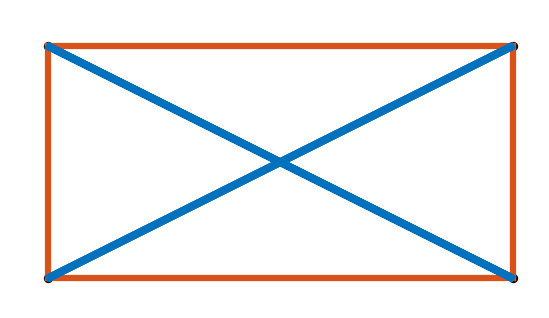
generated by the code

from tnsgrt.plotter.matplotlib import MatplotlibPlotter
plotter = MatplotlibPlotter()
plotter.plot(s)
fig, ax = plotter.get_handles()
ax.view_init(90,-90)
ax.axis('equal')
ax.axis('off')
plt.show()

Properties

Node and member properties are stored as pandas’ Dataframes. In this example

s.node_properties

returns the dataframe:

   radius  visible constraint          facecolor          edgecolor
 0.002     True       None  (0, 0.447, 0.741)  (0, 0.447, 0.741)
 0.002     True       None  (0, 0.447, 0.741)  (0, 0.447, 0.741)
 0.002     True       None  (0, 0.447, 0.741)  (0, 0.447, 0.741)
 0.002     True       None  (0, 0.447, 0.741)  (0, 0.447, 0.741)

and

s.member_properties

returns:

   lambda_  force  stiffness  volume  radius  inner_radius  mass  rest_length
    0.0    0.0        0.0     0.0   0.005           0.0   1.0          0.0  \
    0.0    0.0        0.0     0.0   0.005           0.0   1.0          0.0
    0.0    0.0        0.0     0.0   0.005           0.0   1.0          0.0
    0.0    0.0        0.0     0.0   0.005           0.0   1.0          0.0
    0.0    0.0        0.0     0.0   0.010           0.0   1.0          0.0
    0.0    0.0        0.0     0.0   0.010           0.0   1.0          0.0

           yld  density       modulus  visible             facecolor
250000000.0   7850.0  2.000000e+11     True  (0.85, 0.325, 0.098)  \
250000000.0   7850.0  2.000000e+11     True  (0.85, 0.325, 0.098)
250000000.0   7850.0  2.000000e+11     True  (0.85, 0.325, 0.098)
250000000.0   7850.0  2.000000e+11     True  (0.85, 0.325, 0.098)
250000000.0   7850.0  2.000000e+11     True     (0, 0.447, 0.741)
250000000.0   7850.0  2.000000e+11     True     (0, 0.447, 0.741)

              edgecolor  linewidth linestyle
(0.85, 0.325, 0.098)          2         -
(0.85, 0.325, 0.098)          2         -
(0.85, 0.325, 0.098)          2         -
(0.85, 0.325, 0.098)          2         -
   (0, 0.447, 0.741)          2         -
   (0, 0.447, 0.741)          2         -

The DataFrames can be manipulated directly or one can use convenience methods that will be discussed later.

Properties are populated with default values taken from Structure.NodeProperty, Structure.MemberProperty, and the values in the dictionary

Structure.member_defaults

returns the dictionary:

{'bar': {'facecolor': (0, 0.447, 0.741), 'edgecolor': (0, 0.447, 0.741)},
 'string': {'facecolor': (0.85, 0.325, 0.098),
  'edgecolor': (0.85, 0.325, 0.098),
  'radius': 0.005}}

The keys in this dictionary are tags, which we discuss next.

Tags

Nodes and members can be assigned and manipulated via tags. Nodes do not have any default tag, as

s.node_tags

returns:

{}

but members are automatically assigned either bar or string as a tag. Typing

s.member_tags

returns:

{'bar': array([4, 5], dtype=int64), 'string': array([0, 1, 2, 3], dtype=int64)}

This association happens at the constructor time by passing the parameter number_of_strings, which tags the first number_of_strings members as strings and the remaining as bars. Alternatively, one can pass tags at construction time in the form of a dictionary with tags as keys and a numpy array of node or string indices as values.

It is always recommended to manipulate tags using the convenience methods of tnsgrt.structure.Structure, which take care of keeping the member and node indices unique and sorted.

Additional member tags can be assigned using tnsgrt.structure.Structure.add_member_tag(). For example

s.add_member_tag('vertical', [0, 2])

creates a new tag vertical and associated the two members with indices 0 and 2 to it. Conversely, tnsgrt.structure.Structure.get_members_by_tag retrieves the member indices associated with a given tag, as in

s.get_members_by_tag('vertical')

which returns:

array([0, 2])

while tnsgrt.structure.Structure.get_member_tags retrieve all tags associated with a given member index:

s.get_member_tags(2)

which returns:

['string', 'vertical']

Similar methods exist to manipulate node tags.

Member and node properties

Even though it is possible to manipulate the property DataFrames directly, it is often easier to use the provided convenience methods.

For example

s.get_member_properties(s.get_members_by_tag('vertical'), 'radius', 'facecolor', 'edgecolor')

retrieves a view of the member’s properties:

   radius             facecolor             edgecolor
0   0.005  (0.85, 0.325, 0.098)  (0.85, 0.325, 0.098)
2   0.005  (0.85, 0.325, 0.098)  (0.85, 0.325, 0.098)

for all members that have vertical as a tag.

Conversely

s.set_member_properties(s.get_members_by_tag('vertical'), 'radius', 0.04)

sets the radius property of the members that have vertical

tnsgrt.structure.Structure.set_member_properties() can also be used to set multiple values at the same time, as in

from tnsgrt.utils import Colors

s.set_member_properties(s.get_members_by_tag('vertical'),
                      'facecolor', Colors.GREEN.value,
                      'edgecolor', Colors.GREEN.value,
                      'mass', 2)

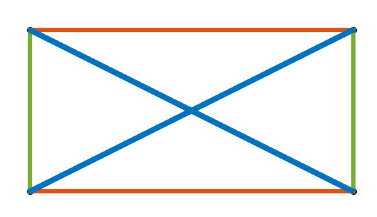
Retrieving the properties confirm the changes:

s.get_member_properties(s.get_members_by_tag('vertical'), 'radius', 'mass', 'facecolor', 'edgecolor')

in the dataframe:

   radius  mass              facecolor              edgecolor
0    0.04   2.0  (0.466, 0.674, 0.188)  (0.466, 0.674, 0.188)
2    0.04   2.0  (0.466, 0.674, 0.188)  (0.466, 0.674, 0.188)

These changes are also reflected on the structure’s plot generated by the following code.

plotter = MatplotlibPlotter()
plotter.plot(s)
fig, ax = plotter.get_handles()
ax.view_init(90,-90)
ax.axis('equal')
ax.axis('off')
plt.show()