Examples
Minimal Snelson 3-Prism
The default constructor of tnsgrt.prism.Prism
from tnsgrt.prism import Prism
s = Prism()
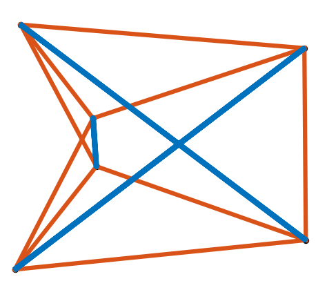
produces a minimal Snelson 3-Prism, with 3 bars, 3 top and 3 bottom strings, 3 vertical strings, and a twist angle of 30 degrees, as in:
which is generated by the code:
import numpy as np
from matplotlib import pyplot as plt
from tnsgrt.plotter.matplotlib import MatplotlibPlotter
%matplotlib widget

plotter = MatplotlibPlotter()
plotter.plot(s)
fig, ax = plotter.get_handles()
ax.view_init(elev=20, azim=45)
ax.axis('off')
plt.show()
The twist angle is the angle measured between the rotations of the top and bottom triangles, which can be better visualized from a different view point

as produced by the following code:
ax.view_init(elev=90, azim=-90)
ax.axis('off')
ax.plot([0, 1.1], [0, 0], 'r--')
ax.plot([0, 1.1*np.cos(np.pi/6)], [0, 1.1*np.sin(np.pi/6)], [1, 1], 'r--')
ax.text(1.1*np.cos(np.pi/12), 1.1*np.sin(np.pi/12), 0, 'alpha')
plt.show()
For a symmetric prism, the 30 degrees twist angle is the only possible equilibrium:
s.equilibrium()
which imparts bars and vertical strings the same magnitude of force coefficient:
s.member_properties[['lambda_']]
lambda_ |
|
|---|---|
0 |
0.57735 |
1 |
0.57735 |
2 |
0.57735 |
3 |
0.57735 |
4 |
0.57735 |
5 |
0.57735 |
6 |
1.00000 |
7 |
1.00000 |
8 |
1.00000 |
9 |
-1.00000 |
10 |
-1.00000 |
Minimal Snelson Prisms have at least one soft mode, which can be confirmed by calculating the model stiffness with rigid body constraints
s.update_member_properties(['stiffness'])
stiffness, _, _ = s.stiffness(apply_rigid_body_constraint=True)
and evaluating its eigenvalues
d, v = stiffness.eigs()
d
which in this case are:
2.77128123e+00
4.68096753e+06
4.68096753e+06
1.23281719e+07
1.23281719e+07
2.45882799e+07
2.72069922e+07
2.89745460e+07
2.89745460e+07
6.68906843e+07
6.68906843e+07
8.82860836e+07
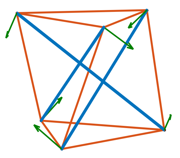
The corresponding eigenvector is plotted below:
as produced by the following code:
V = v[:,0].reshape((3, 6), order='F')

plotter = MatplotlibPlotter()
plotter.plot(s)
fig, ax = plotter.get_handles()
ax.quiver(s.nodes[0,:], s.nodes[1,:], s.nodes[2,:], V[0,:], V[1,:], V[2,:], arrow_length_ratio=.2, color='g')
ax.view_init(10,20)
ax.axis('off')
plt.show()
The plot suggests that the soft mode is associated with a “corkscrew” like rotational motion of the structure.
The presence of this soft mode means that one should expect large displacements in response to compressive type forces such as:
f = 0.25*np.array([[0,0,1],[0,0,1],[0,0,1],[0,0,-1],[0,0,-1],[0,0,-1]]).transpose()
The corresponding approximate displacement can be obtained as:
x = stiffness.displacements(f)
x
which are:
+3.70368807e-09  3.12499981e-02 -3.12500018e-02 -1.80421927e-02 -1.80421991e-02  3.60843918e-02
-3.60843918e-02  1.80421991e-02  1.80421927e-02  3.12500018e-02 -3.12499981e-02 -3.70368809e-09
+1.80422060e-02  1.80422060e-02  1.80422060e-02 -1.80422060e-02 -1.80422060e-02 -1.80422060e-02
Comparing the magnitude of the force with the magnitude of the displacement in the direction of the force
np.sum(f * x, axis=0)/np.linalg.norm(x, axis=0)**2
one obtains:
2.77128222 2.77128222 2.77128222 2.77128222 2.77128222 2.77128222
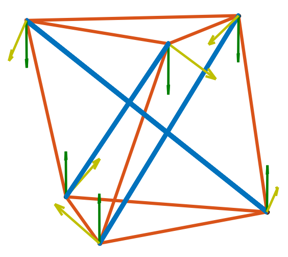
from which we can observe the impact of the soft mode on the structure response. The displacements, scaled 10 times, are visualized along with the applied forces in the figure:
as produced by the following code:
X = f
Y = 1e1*x

plotter = MatplotlibPlotter()
plotter.plot(s)
fig, ax = plotter.get_handles()
ax.quiver(s.nodes[0,:], s.nodes[1,:], s.nodes[2,:], X[0,:], X[1,:], X[2,:], arrow_length_ratio=.2, color='g')
ax.quiver(s.nodes[0,:], s.nodes[1,:], s.nodes[2,:], Y[0,:], Y[1,:], Y[2,:], arrow_length_ratio=.2, color='y')
ax.view_init(elev=10, azim=20)
ax.axis('off')
plt.show()
Non-minimal Snelson 3-Prism
With the addition of diagonal strings, Snelson 3-prisms can be constructed that are in equilibrium at twist angles other than 30 degrees. The following syntax
s = Prism(alpha=np.pi/5, diagonal=True)
produces one such prism. The indices of the additional diagonal strings
can be obtained by searching for the tag ‘diagonal’:
diagonals = s.get_members_by_tag('diagonal')
We can use these indices to set a different color for the diagonal strings
from tnsgrt import utils
s.set_member_properties(diagonals, 'facecolor', utils.Colors.GREEN.value, wrap=True)
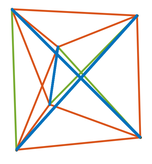
The resulting prism is visualized below:
as produced by the code:
plotter = MatplotlibPlotter()
plotter.plot(s)
fig, ax = plotter.get_handles()
ax.view_init(elev=20, azim=45)
ax.axis('off')
plt.show()
Note the presence of the additional diagonal strings in green.
Equilibrium of the prism and the member stiffness can be calculated as before:
s.equilibrium()
s.update_member_properties(['stiffness'])
Next we calculate the model stiffness with rigid body constraints and its eigenvalues
stiffness, _, _ = s.stiffness(apply_rigid_body_constraint=True)
d, v = stiffness.eigs()
d
to obtain:
8155119.28425745
8155119.32734769
10724386.65730408
22597331.51554979
22597331.53389546
23044828.36153938
27206992.10546769
31904308.56966601
31904308.58628615
67275457.78066988
67275457.82203464
96162998.90710124
Note that there are no soft modes and the associated displacement in response to a compressive force is
x = stiffness.displacements(f)
x
which equals:
 4.67852301e-09  2.69664424e-09 -7.37516722e-09  3.67055126e-10 -6.63920203e-09  6.27214688e-09
-5.81496304e-09  6.95920134e-09 -1.14423828e-09  7.45437076e-09 -3.40930636e-09 -4.04506442e-09
 1.20433838e-08  1.20433839e-08  1.20433839e-08 -1.20433839e-08 -1.20433839e-08 -1.20433838e-08
The corresponding stiffness in the direction of the applied force is
np.sum(f * x, axis=0)/np.linalg.norm(x, axis=0)**2
which is equal to:
14998326.01216395 14998325.9409232 14998325.99099865 14998325.98357238 14998325.94372185 14998326.01679158
These are orders of magnitude higher than the displacement of the same minimal version of the prism, which was soft.
The displacements, scaled \(10^7\) times, are visualized along with the applied forces in the figure:
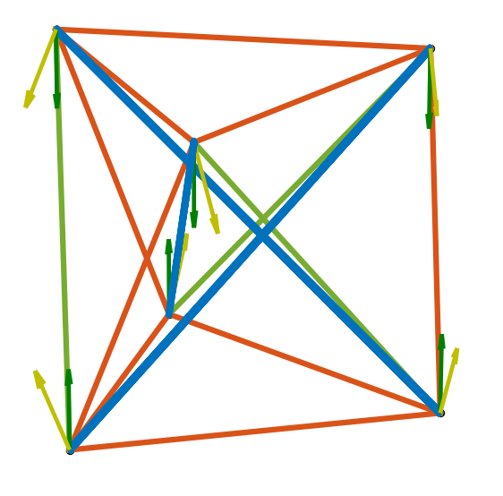
generated by the code:
X = f
Y = 2e7*x

plotter = MatplotlibPlotter()
plotter.plot(s)
fig, ax = plotter.get_handles()
ax.quiver(s.nodes[0,:], s.nodes[1,:], s.nodes[2,:], X[0,:], X[1,:], X[2,:], arrow_length_ratio=.2, color='g')
ax.quiver(s.nodes[0,:], s.nodes[1,:], s.nodes[2,:], Y[0,:], Y[1,:], Y[2,:], arrow_length_ratio=.2, color='y')
ax.view_init(elev=20, azim=45)
ax.axis('off')
plt.show()
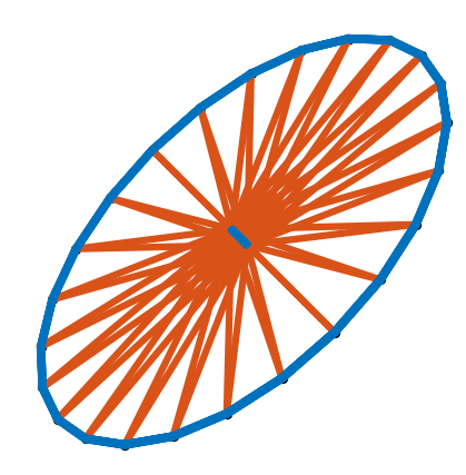
Bicycle wheel
In this example we will build a structure to illustrate how to combine simple modules into a larger structure. The goal is to build a tensegrity structure that resembles a bicycle wheel as in the following figure:
The wheel is parametrized by the following constants:
\(r\): the wheel radius;
\(n\): the number of sides of the “rim”;
\(h\): the height of the central “hub”,
which are defined below:
r = 1
h = .1
n = 24
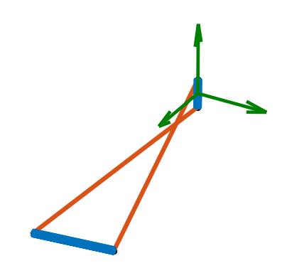
We are going to break the design up into a series of similar units. Each unit consists of two bars and two strings. One bar is the wheel central “hub”, aligned with the z-axis, and the other bar is a segment of the “rim,” which lies on the x-y plane. The two strings make up the wheel “spokes”, each one connecting one node from the “hub” to the end of the “rim” bar. We build such a unit as follows:
nodes = np.array([[0, 0, -h/2], [0, 0, h/2], [r, 0, 0], [r*np.cos(2*np.pi/n), r*np.sin(2*np.pi/n), 0]]).transpose()
strings = np.array([[0, 2], [1, 3]]).transpose()
bars = np.array([[0, 1], [2, 3]]).transpose()
members = np.hstack((strings, bars))
member_tags = {'hub': 2, 'rim': 3}
The tags 'hub' and 'rim' will later help us track those elements
in the complete wheel. The resulting unit is the following Structure:
from tnsgrt.structure import Structure
unit = Structure(nodes, members, member_tags=member_tags, number_of_strings=strings.shape[1])
unit
which is visualized in the figure generated by the following code which includes a frame at the origin for reference:
plotter = MatplotlibPlotter()
plotter.plot(unit)
_, ax = plotter.get_handles()
ax.view_init(elev=30, azim=30, roll=0)
ax.quiver([0, 0, 0], [0, 0, 0], [0, 0, 0], [1/4, 0, 0], [0, 1/4, 0], [0, 0, 1/4], color='g')
ax.axis('off')
ax.axis('equal')
plt.show()
Now imagine rotating this unit about the z-axis to build up the entire wheel. This is done below:
from tnsgrt import structure

wheel = Structure()
theta = 2*np.pi/n
for i in range(n):
  wheel.merge(structure.rotate(unit, i*theta*np.array([0, 0, 1])))
resulting in a structure with \(4 n\), \(2 n\) bars, and \(2 n\) strings
Of course, in building the above structure, we have also created
\(n\) copies of the central hub and coincident nodes at the edge
of each rim member, which makes a total of \(2 (n-1) + n\)
redundant nodes. Those redundant nodes can be merged using
tnsgrt.structure.Structure.merge_close_nodes():
wheel.merge_close_nodes()
which reduces the total number of nodes from \(4 n\) to
\(n + 2\). Yet, there are still \(2 n\) bars, with \(n\)
of those being copies of the central hub. After using the method
tnsgrt.structure.Structure.merge_overlapping_members()
wheel.merge_overlapping_members()
the number of bars reduces to \(n + 1\). Since none of the strings overlap, they were not merged. The result of these merging operations left the structure with a single hub member
wheel.get_members_by_tag('hub')
which returns:
array([2])
and \(n\) rim members
wheel.get_members_by_tag('rim')
which returns:
array([ 3,  6,  9, 12, 15, 18, 21, 24, 27, 30, 33, 36, 39, 42, 45, 48, 51,
       54, 57, 60, 63, 66, 69, 72])
The final product is visualized below:
plotter = MatplotlibPlotter()
plotter.plot(wheel)
_, ax = plotter.get_handles()
ax.view_init(elev=30, azim=0, roll=45)
ax.axis('off')
ax.axis('equal')
plt.show()
For those who might be surprised by the fact that a wheel can be built out of a rim that is not a single rigid unit, we verify the stability of the design by calculating equilibrium under pretension
wheel.equilibrium()
and evaluating the stiffness of the model after updating the model’s material properties
wheel.update_member_properties()
stiffness, _, _ = wheel.stiffness(apply_rigid_body_constraint=True)
The smallest eigenvalues of the stiffness matrix are indeed positive
d, v = stiffness.eigs()
d[:12]
which returns:
array([78242.18249671, 78242.2522954 , 78242.25229541, 78242.45693482,
       78242.45693486, 78242.78246912, 78242.78246913, 78243.20671369,
       78243.2067137 , 78243.70075696, 78243.70075701, 78244.23093071])
indicating that the structure is in a stable equilibrium under pretension. The individual member forces at equilibrium are shown below:
wheel.get_member_properties(wheel.get_members_by_tag('hub'), 'force')
to be equal to:
-0.041879
at the hub,
wheel.get_member_properties(wheel.get_members_by_tag('rim'), 'force')
to be equal to:
3    -0.267374
6    -0.267374
9    -0.267374
12   -0.267374
15   -0.267374
18   -0.267374
21   -0.267374
24   -0.267374
27   -0.267374
30   -0.267374
33   -0.267374
36   -0.267374
39   -0.267374
42   -0.267374
45   -0.267374
48   -0.267374
51   -0.267374
54   -0.267374
57   -0.267374
60   -0.267374
63   -0.267374
66   -0.267374
69   -0.267374
72   -0.267374
Name: force, dtype: float64
at the rim members, and
wheel.get_member_properties(wheel.get_members_by_tag('string'), 'force')
to be equal to:
0     0.034943
1     0.034943
4     0.034943
5     0.034943
7     0.034943
8     0.034943
10    0.034943
11    0.034943
13    0.034943
14    0.034943
16    0.034943
17    0.034943
19    0.034943
20    0.034943
22    0.034943
23    0.034943
25    0.034943
26    0.034943
28    0.034943
29    0.034943
31    0.034943
32    0.034943
34    0.034943
35    0.034943
37    0.034943
38    0.034943
40    0.034943
41    0.034943
43    0.034943
44    0.034943
46    0.034943
47    0.034943
49    0.034943
50    0.034943
52    0.034943
53    0.034943
55    0.034943
56    0.034943
58    0.034943
59    0.034943
61    0.034943
62    0.034943
64    0.034943
65    0.034943
67    0.034943
68    0.034943
70    0.034943
71    0.034943
Name: force, dtype: float64
at all “spoke” strings.